The BARRINGER PROCESS RELIABILITY Course
Get a 20% discount on this course if you purchase before 31st December, 2025!
Use the coupon: BPR-20 on checkout to redeem this discount!
Lesson 1 - Course Contents and introduction to the SuperSMITH® Software
This Lesson provides a brief but comprehensive overview of BPR including its practical applications. The course content is listed as well as all the theoretical concepts covered. This also includes the perquisites and best suited audience for the course. The Super SMITH® software required to do a BPR Analysis, is introduced. This includes the Super SMITH® license purchase, technical support and user documentation. (Lesson Duration: 1 hour 15 minutes)
Section 1 – “Flyover” of BPR
This section is a detailed A to Z summary of everything covered during this course. This includes a practical example showcasing BPR and its output. Essentially from getting the production records all the way to having a production performance report. (Section Duration: 22 minutes)
Section 2 – Course Outline and Requirements
This section contains the course summary, prerequisites, and general user experience (Section Duration: 19 minutes)
Section 3 - The BPR Software - Super SMITH® Overview
This section contains a detailed overview of the Super SMITH® Software. This includes Purchasing, Support Documentation, and the Platform Development Team. It also includes information on the New Weibull Handbook as well as an overview of the weibullnews.com website which contains additional information on reliability engineering and other free resources. (Section duration: 19 minutes)
Section 4 - SuperSMITH® basic manipulation
This section provides an overview of the Super SMITH® Software functionality specifically related to conducting a BPR analysis. This includes icon setup, data entry and plotting. Only the Weibull Module is covered as it is where the BPR functionality resides. (Section duration: 15 minutes)
Lesson 2 - Reliability Engineering and BPR Fundamentals
This lesson provides an overview of the theoretical concepts that make up BPR. We learn about the “negative” paradigms and production mindsets in industry that can be altered by BPR. The fundamentals of Reliability Engineering as a science are introduced as well as the Weibull Distribution. As the BPR concept is essentially based on the Weibull Distribution. There is also an overview supported by examples, of Traditional Reliability Analysis versus Strategic Reliability Analysis. BPR is a Strategic Analysis. That is a high-level overview of a production plant, hence a management tool. (Lesson Duration: 1hr 19minutes)
Section 1 – BPR and Common Industry Paradigms
This section reviews the paradigms and production mindsets in industry that can be altered by BPR. The concept of variability in production is introduced as it is very often overlooked. The “hidden factory” remains unseen and therefore unaddressed because production personnel or management bury their “heads in the sand”. By seeking to uncover variability and the related losses, BPR can guide the organization towards improved performance and profitability. (Section duration: 16 minutes)
Section 2 – Reliability Engineering Concepts
This section introduces the science of Reliability Engineering. The term “Reliability” is often misunderstood and misinterpreted in industry hence the need to define its true meaning. Also, how it is calculated using Statistical Distributions. The Weibull Distribution is the Statistical Distribution that best models production performance hence is the basis of a BPR analysis. Its characteristics and main attributes are explained here. (Section Duration: 20 minutes)
Section 3 - The Weibull distribution applied to Production Analysis
This section looks at the difference between the Six Sigma methodology and BPR. Six Sigma being a well-established production and quality analysis, what makes BPR stand out? We also review the difference between Traditional Reliability and BPR. Traditional Reliability goes in the “weeds” of system hence is more complex, whereas BPR is more strategic. Both are important in Reliability Engineering but have different scopes and objectives. Also demonstrated in this lesson, is why the Weibull Distribution best represents production performance versus the Normal Distribution used in Six Sigma. (Section Duration: 21 minutes)
Section 4 - Gathering all the above in BPR
This section is a summary of all the concepts we have learnt in Lesson 2. A BPR analysis is a combination of visuals, through graphs, as well as numerical outputs. The Weibull statistics provide us with ONE number for variability as well as a production target or “bulls-eye” to aim for every day. We also understand how much control we have on the process as well as the productions losses. All of this on ONE single sheet of paper! The lesson also reviews the systemic problems we should address once the BPR analysis is completed as well as how to tackle both Reliability (Crash and Burn) and Nameplate losses. (Section duration: 22 minutes)
Lesson 3 - Practical Session - BPR Plot Construction
The lesson is purely practical. It allows to learner to build a BPR plot from scratch using the SuperSMITH® Software. The lesson progresses through the more complex aspects and towards the end, a reporting process is suggested. This will enable the BPR analyst to communicate their findings to an audience in a structured, comprehensive yet effective manner. (Lesson duration: 1 hour 27 minutes)
Section 1 – The required inputs to a BPR Analysis
This section provides the practical and hands-on knowledge on how to build a basic probability plot in the Super SMITH® Software. This is the first step towards building a BPR plot. The rain plot construction and its limitations are also covered. Both plots use production records from an MS Excel® spreadsheet. (Section Duration: 20 minutes)
Section 2 – Step-by-Step Construction of the BPR Plot in SuperSMITH® (Part 1)
This section provides the practical and hands-on knowledge on how to add the specific BPR elements to the probability plot built in Section 1 using the Super SMITH® Software. Those include the Demonstrated Production Line and the Process Reliability Point. (Section Duration: 25 minutes)
Section 3 - Advanced construction of the BPR Plot - Part 2
Having constructed the Demonstrated Production Line and The Process Reliability Point in the previous Section 2, we can now build a first report on our existing BPR plot. Moving from graphical views provided by the BPR plot, we will now have quantified results on performance. The completion of the report will be done in the next Section 4. This section also looks in depth at the variability concept or beta value with illustrated examples. Finally we will construct our Nameplate Line which is the last element of our BPR plot. (Section Duration: 25 minutes)
Section 4 - BPR plot interpretation and reporting
Having constructed the Nameplate Line in Section 3, this section will showcase how the Nameplate or Efficiency and Utilisation losses are calculated from the BPR plot. Having all the BPR elements now constructed, we will be able to extract a final numerical report on the overall performance. This is followed by a process to present the results to an audience. As well as how to initiate a continuous improvement program using all the information gathered so far. (Section Duration: 17 minutes)
Lesson 4 - Advanced BPR Analysis
This lesson provides practical knowledge of 3 applications of the BPR Analysis. In previous lessons we learned how to build a BPR analysis. Now we move on to using the analysis for specific purposes such as Cutback Loss Analysis and Benchmarking. The last section involves gathering random records to build a BPR analysis when none is available. This is based on the Monte-Carlo simulation method with is a fundamental concept in Reliability Engineering. (Section duration: 1 hour 1 minute)
Section 1 – Cut Back Losses
This section highlights another type of loss category found in BPR analysis. Cutback losses are losses that occur periodically during an operation. They have a specific signature pattern on the BPR plot. And can be quantified precisely. (Section Duration: 22 minutes)
Section 2 – Comparing Performance and Benchmarking between factories using BPR
This section looks at comparing different production performances. This involves putting multiple BPR plots on the same graph. The comparison could be chronological or between different plants. (Section Duration: 24 minutes)
Section 3 - BPR Data Generation using Monte Carlo Simulations
This final section teaches the learner how generate BPR plots from scratch using the Monte Carlo simulation feature in the SuperSMITH® software. The Monte Carlo process is a very common tool in Reliability Engineering providing random numbers from predefined statistical distributions. In our case, a two parameter Weibull Distribution. (Section Duration: 15 minutes)

Core Speciality: Reliability Analysis and Block Diagram Modelling
Target customers: Industrial operations seeking to quantify the future performance of their assets in order to optimize financial budgets, production output and resource allocations (capital, work force, spare parts, etc.).
Definition of Reliability Modelling
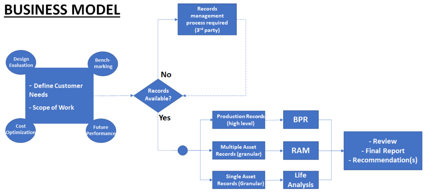
Also known as Reliability, Availability and Maintainability (RAM) Modelling, this concept breaks down an operation or system into significant blocks and quantifies the interactions and ultimate contribution of each block to the total output of the operation (e.g. m3 of finished product, manufactured goods, mining ore, etc).
Once established, the model can inform the operator on various improvement opportunities related to each block including availability bottlenecks, maintenance optimization, spares parts management or maintenance resource allocation. The RAM model is also a tool of choice to estimate the benefits of changes to an operation
(e.g. adding redundancy) as it is cheaper to review the change on paper rather than in real life.
Definition Reliability Analysis
Two types of Reliability analysis are offered as follows:
1) Life analysis often known as “Weibull analysis”: The concept uses statistical tools to define life characteristics of assets or components. Using historical variables such as operating time, odometer km or on/off cycles, one can define characteristics of equipment informing an operator of the future number of failures, probabilities of failures or define the bathtub curve characteristics of an asset.
2) Barringer Process Reliability: this concept is defined as a 10,000 ft overview of an operation and uses only production output data such as barrels per day, widgets produced per day etc. It is essentially a
management tool and can help the operator establish the operating characteristics of the asset as well as the real losses experienced by the asset. It can also be used as a benchmarking tool if for example
an operator has multiple production sites or several identical processing units on one site.
The fine print: The statistical analysis is based on the information and records provided by the client. The analysis provides guidance to what the asset(s) studied is expected to perform in the future based on past performance but does not guarantee any outcomes. It is strongly recommended that the client review the report and recommendations with subject matter experts to make final decisions.
Want to ask Cogito Reliability a question? Fill out the form below.
But what is Reliability Engineering?
Reliability Engineering is an established science with rigorous concepts involving mathematical and statistical methods, and those can often appear daunting for some maintenance or risk practitioners. The role of the reliability engineer is to master, explain, and apply those concepts as well as work with peers to make the correct decision(s) regarding the maintenance of operating assets or future design capabilities. Those decisions are crucial, especially when it comes to the safety of frontline workers, capital investments, or the preservation of the environment. To use my fellow Reliability Engineer, Fred Shenkelberg’s1 own terms, the Reliability Engineer asks two simple questions:
- What will make the equipment fail?
- When will the equipment fail?
I have outlined 9 themes below as well as what "data" or information is required from the customer to do this. The fine print: all those reliability calculations are based on historical complete (clean) records provided by a customer. Changes in performance based on unknown events can occur and modify future performance. The statistical analysis provided to the customer is intended to guide their decision based on the likely but NOT guaranteed turnout of events.
1) What is the expected number of failures in a defined future interval of time on a specific asset or set of assets generally of the same type (e.g. cooler pumps).
The customer wants to know how many events he will have to deal with in the coming months or years so he can organize his resources (spare parts, labour, $ budgets, etc).
This requires a reliability study to develop a life model for the typical asset. The inputs to the study are failure/repair records (typically dates) and equipment start date. See Maintrain 2020 paper (on my website) for more details on this. The more detailed the customer records the better - sparse and incomplete records are difficult to work with though not impossible; otherwise have to default to literature-based models IF available but this might lead to approximative results. This study also gives the customer an idea on how "fast" the asset is deteriorating.
2) What is the economical number of spare parts we should have in our spares/supply chain inventory?
Spares are expensive and to get them to sit unused in our stores is wasting $$$. On the other hand, if we don't have them when we need them it can cost us downtime hence revenue $$$.
In order to find the optimal/most economical number of spares to keep in stock we must do a study as in 1) above on the asset and the apply the cost optimization technique. The inputs to the study are failure/repair records (typically dates), equipment start/commissioning dates, cost of repairs/maintenance and finally cost of downtime (typically lost production revenue). We also need to know the logistics to get spares in stock. This is also the technique we use to get spares min/max levels. Once this model is built, we can work with vendors to see how we can improve logistics or costs - e.g. keep spares on vendor sites rather than customer's warehouse.
3) When is it most economical to replace this asset with a new one?
Assets age and cost us more money over time in terms of repairs or loss of efficiency. However, if replaced too early that can be expensive especially if the replacement costs are high. If done too late it can cost us $ in terms of lost production especially if it is a catastrophic failure. We have to calculate the optimal time when the risk and costs are minimized. The same technique is used as in 2) above (i.e. economical replacement time). Similarly, we can calculate overhaul timing with this technique - when is the best time to send equipment for overhaul.
4) What is the economical benefit (or lack of thereof) of adding redundant/standby/spare equipment in order to a process.
Equipment failures can bring significant impact to a process especially if this equipment is a single point vulnerability (i.e. if it fails the entire process comes down). Redundancy can be a solution to the problem but it has to be carefully assessed especially if we are dealing with expensive retrofits. Redundancy would mean adding an identical unit in the process whereby if one unit fails, the other identical unit immediately takes over minimizing downtime production impact - the failed item can be repaired and brought back to a functional / stand-by-state. The Reliability technique used here is specifically described in the 2022 Maintrain Paper. It would require the typical CMMS records from the customer as well as production downtime costs and more importantly an accurate and complete cost of adding the redundant unit. We end up with a RAM model. A risk analysis process is also recommended to ensure the new unit does not result in undesirable outcomes like controls, process or hydraulic issues typically not covered by a reliability study.
5) Based on the current performance, what is the expected production output of the production unit or entire plant in a future interval of time?
Operators build a production plant and expect to get full production at the same rates every single day of the year. This is not the case in reality. Equipment fails, incidents happen and we have process quality mishaps which end up causing lower production outputs. Building a RAM model of the production plant including all its "significant" process units and the simulated failures times and impacts can help visualize the operation of the plant in a more realistic view. The RAM model output therefore can provide the most realistic performance (bbls, widgets, tonnes or ore, etc) of the plant say in the next 5,10, 20 years, etc. This can also highlight known bottlenecks and quantify their overall impact including production, maintenance costs and downtime. The RAM model should also include information about the operating philosophy of the plant or production unit (how it is used, % time used, turn ups or turn down proportion etc). If the plant has been in production for a while and has detailed output records, the BPR technique defined in the 2022 Maintrain Paper can be used. However this does not provide as detailed information as the RAM model yet is way much easier to build compared to a RAM model.
6) If this asset has survived to date without any catastrophic failure, what is the probability that it will survive another two years as this is how long it will take for us to replace it as well as find the $ budget.
This is used for critical assets that if they fail, will cause significant impact on production. Additionally, those assets cost a significant amount of $ to replace and have a long lead time as they are custom built and not an off the shelf item. For example, this could be a power transformer on an oil pipeline which takes two years to replace at a cost 10+ million dollars. Finding the probability of failure in the next short time interval (e.g. 2 years away) is a way to gauge the risk* and hence how long we can wait before the asset is replaced (Risk* = probability x consequence) . This probability is derived from the same analysis performed in 1) above. On a side note, just to point out that a Reliability Life Analysis on an asset can provide multiple answers to a customer so it is a very valuable and versatile process.
7) What is the maintenance strategy for this set or population of assets?
Maintrain Paper 2021 (Page 8) on my website gives an idea on how to develop part of a maintenance strategy that will enhance the availability of an asset or population of assets. The reliability calculations are the basis of this strategy but the implementation feasibility of the strategy should always be vetted by the customer. Another tool that is used to define a maintenance strategy is FMEAs (Failure Modes and Effects Analysis - a team driven process a bit like HAZOPs or PHAs). The Reliability Engineer in collaboration with other specialties, helps define a maintenance strategy that is based on the asset's historical performance rather than from a vendor's manual. The maintenance strategy can involve inspections, advanced condition monitoring or preventive replacements of components. The fundamental inputs to an optimal maintenance strategy are good equipment records and detailed knowledge of the asset (how it works and how it fails).
8) Can we quantify the bottle neck impact in a process (i.e. how much is the equipment that is causing problems really costing us in terms of repairs or revenue loss)?
Operators often know what is causing them losses in their process but the challenge is to quantify this loss in production units, revenue $$$ or downtime. This question works in conjunction with question 5. We have built a RAM model for the process where the "culprit" is included. We have to run the model for a desired interval (e.g. 5 years) and drill down to the bottle neck's contribution to lost revenue, downtime etc.
9) Big Vice President in Big Office want to know how his operation is doing on “one sheet of paper” without going into details of what’s broken
Barringer Process Reliability (or BPR) is a great tool for this. It needs minimal inputs and uses to the Weibull statistical process to define simple KPIs that highlight the performance of a plant or operation. It can also be used as a benchmarking tool if for example an operator has multiple production sites or several identical processing units on one site.


